Dimensionality reduction is an important technique to overcome the curse of dimensionality in data science and machine learning. As the number of predictors (or dimensions or features) in the dataset increase, it becomes computationally more expensive (ie. increased storage space, longer computation time) and exponentially more difficult to produce accurate predictions in classification or regression models. Moreover, it is hard to wrap our head around to visualize the data points in more than 3 dimensions.
How do we reduce the number of features in dimensionality reduction?
We first determine which feature and how much of this feature contributes to the representation of the data and remove the features that don’t contribute much to the representation of the data.
This article will review the linear technique for dimensionality reduction, in particular, principal component analysis (PCA) and linear discriminant analysis (LDA) in scikit learn using the wine dataset (available HERE).
Let’s say our dataset has d number of independent or feature variables (dimensions). It is not feasible to visualize our data if it contains more than 2 or 3 dimensions. Applying PCA on our dataset will allow us to visualize the result since PCA will reduce the number of dimensions and extract k dimensions (k<d) that explain the most variance of the dataset. In other words, PCA reduces the dimensions of a d-dimensional dataset by projecting it onto a k-dimensional subspace, where k < d.
PCA is an unsupervised linear transformation technique: although PCA learns the relationship between dependent and independent variables to find a list of principal components, we do not consider the dependent variable in the model.
Unlike PCA, LDA extracts the k new independent variables that maximize the separation between the classes of the dependent variable. LDA is a supervised linear transformation technique since the dependent variable (or the class label) is considered in the model.
TAKEAWAY: PCA maximizes the variance in the dataset while LDA maximizes the component axes for class-separation.
Let’s take a look at the wine dataset from UCI machine learning repository. This data examines the quantities of 13 ingredients found in each of the three types of the wines grown in the same region in Italy. Let’s see how we can use PCA and LDA to reduce the dimensions of the dataset.
If you want to follow along, you can download my jupyter notebook HERE for materials throughout this tutorial. Click HERE to look at instructions on how to install jupyter notebook.
Data Preprocessing: Steps to do before performing PCA or LDA
Now, why don’t you click on our wine dataset (click on wine.data)? What do you see?
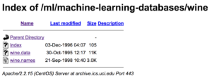
You will notice that the csv file has no specified header names. The first line of the csv is the first data point, not the header.
So, to denote the first line of data, let’s pass in the parameter header and assign None (header=None). For more information on other parameters on pandas.read_csv, click HERE.
![]()
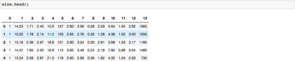
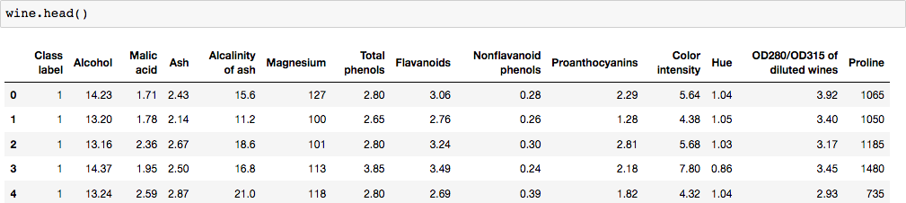
By default, it will print out the first 5 rows.
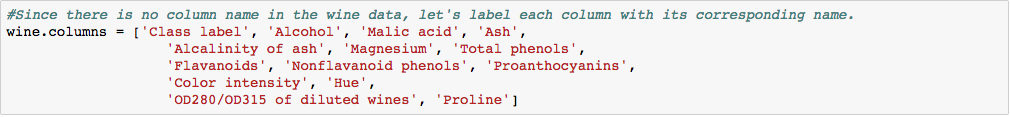
Since our dataset has no header, let’s label each column with its corresponding name.
How do we know what the corresponding column names are?
Click on our wine dataset above and then click on wine.names.
Scroll down to the Relevant Information Section. The first column is the class label (class 1, 2, 3 representing three different wine types). The remaining columns are the 13 attributes shown in this Relevant Information Section.

Now, our columns are labeled.
The first column is the column of interest since it has the ‘Class label’ (or dependent variable or y). We can use iloc for index’s position. Since python is zero-index based, the first column is ‘0’.
The reminding columns include the 13 ingredients present in wine, which are our features (or X).

After defining our X (independent variables) and y (dependent variable), we can split our dataset for training and testing purposes.

Since the 13 variables are measured in different scales, we have to normalize (or standardize) all of them using StandardScaler from sklearn.

After standardizing all the features, we are ready to perform either PCA or LDA.
Let’s perform PCA first.
Principal Component Analysis (PCA)
![]()
We can now pass in the number of principal components; let’s choose 2 components.

We can take a look at the explained variance ratio.

The first component accounts for 36.9% of the variance while the second component accounts for 19.3%.
Now, let’s fit a logistic regression to the training set.

X_test contains the 2 principal components that were extracted and predict the test set result.
![]()
Let’s evaluate the performance of the model by constructing the confusion matrix. We should get a good result since we extracted the 2 principal components that explain the most variance, (60%). In other words, these components were direction of the maximum variance in our dataset.


How should we interpret the result above? Let’s just convert the result above into the following table for an easier interpretation.
| n=36 | Predicted class 1 | Predicted class 2 | Predicted class 3 |
| Actual class 1 | 14 | 0 | 0 |
| Actual class 2 | 1 | 15 | 0 |
| Actual class 3 | 0 | 0 | 16 |
It is a very good result; the diagonal of the table represents the correct predictions. There were 14 cases of correct prediction of class label 1, 15 cases of correct prediction of class label 2, and 6 cases of correct prediction of class label 3. There was one incorrect prediction, where the real outcome was class label 1, but it was predicted to be class label 2.
Accuracy is very good; 35 correct predictions divided by the total number of 36 cases should give us about 97.2% accuracy.
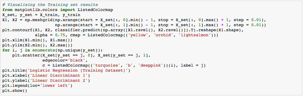
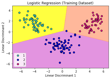
We can visualize our training result as below.
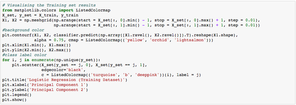
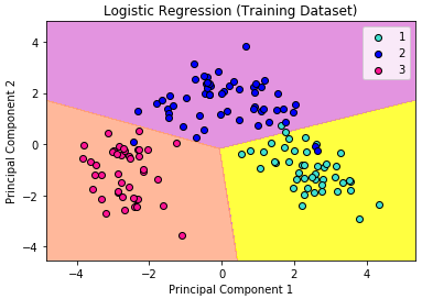
In the visualization above, the color yellow, orchid, and light-salmon color were the predicted regions of class 1, 2, and 3 respectively. The little circles were the real observations in our wine dataset (turquoise=class 1, blue=class 2, deep-pink=class 3).
What we are more interested in is the visualization of our test result. This should be consistent with the evaluation we just obtained from the confusion matrix earlier.
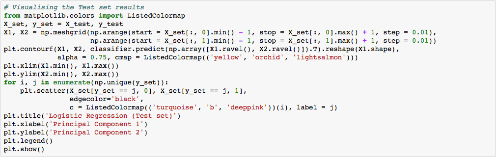
Let’s assess our diagram of the test result. So, we see one blue circle(which is the real outcome for class label 2) but it was predicted to be in the yellow region, which was the class label 1. This was the same incorrect prediction we observed in the confusion matrix above. Overall, using PCA, we are able to obtain ~97% accuracy.
Let’s take a look at how we can apply LDA and whether we can improve the accuracy.
Linear Discriminant Analysis (LDA)
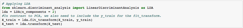
We apply LDA before fitting the classification model to the training set.
*One thing to note is because LDA is a supervised technique, we need to include the dependent variable ‘y_train’ in our model.
The rest of what we do in this section should now be more familiar.


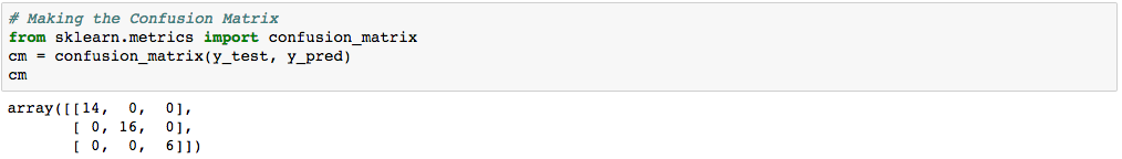
| n=36 | Predicted class 1 | Predicted class 2 | Predicted class 3 |
| Actual class 1 | 14 | 0 | 0 |
| Actual class 2 | 0 | 15 | 0 |
| Actual class 3 | 0 | 0 | 16 |
Were there any incorrect predictions?
NO! HOORAY!
Again, the diagonal of the table represents the correct predictions. There were 14 cases of correct prediction of class label 1, 16 cases of correct prediction of class label 2, and 6 cases of correct prediction of class label 3.
We obtained 100% Accuracy with LDA (36 correct predictions divided by total number of 36 cases).
Let’s visualize our result.
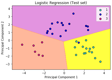
Again, the visualization of our test result should be consistent with the evaluation we just obtained from the confusion matrix earlier.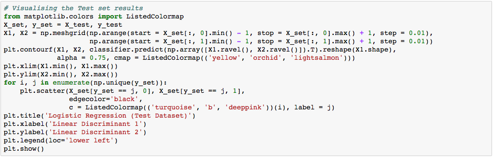
The little circles, which were the real observations in our wine dataset (turquoise=class 1, blue=class 2, deep-pink=class 3), were located in the correctly predicted regions (yellow=class 1, orchid=class 2, and light-salmon=class 3).
In summary, both PCA and LDA performed very well. We reduced from 13 dimensions to 2 and we still got great results for predicting class labels for the 3 different types of wine.
It’s important to note that both PCA and LDA are the dimensionality reduction for linear transformation only. For non-linear transformation, we will need to use kernel-PCA. Stay tuned in the next article.
Takeaway Summary Table:
| PCA | LDA |
| unsupervised | supervised |
| class label is not included | class label is included |
| identify features that account for the most variance in the data | identify features that account for the most variance between classes |
Photo by Jeremy Thomas on Unsplash
Looking for more? Checkout Byte Academy's Data Science Immersive and Intro courses.